Zero-Shot Inference and Relation Vectors
TL;DR
This post tests whether the methodology of Function Vectors can be transferred from in-context learning (ICL) to zero-shot inference. Using a zero-shot prompt, I derive a relation vector through activation patching and ask whether it causally restores the target relation. Although the vector restores correct answers in the correctly-answered subset of Llama-3.2-3B (over 80%), the effect does not generalize to the incorrectly-answered subset (below 40%), to other models, or to another prompt format. These results weaken the initial interpretation that the relation vector captures a robust task mechanism, and instead suggest that the observed success is entangled with model and prompt-specific artifacts.
Motivation
The Function Vectors paper investigated the function vectors of in-context learning (ICL). The paper showed that specific attention heads carry task-relevant information during ICL, and that a compact vector summarizing these heads’ outputs can trigger task execution when injected into the residual stream. However, how LLMs solve problems in zero-shot settings, where no in-context examples are provided, is under-explored.
Core Idea
This experiment follows the same methodology as the paper but uses a different prompt format. Instead of few-shot ICL prompts, two zero-shot prompt formats are used to derive the relation vector.
Prompt format 1: Relation: {relation}\nInput: {input}\nOutput: Prompt format 2: Q: What is the {relation} of {input}?\nA: {output}
The goal is to investigate whether a relation vector derived from zero-shot prompts enforces correct answers in zero-shot inference even when the prompt format is changed. Throughout this post, I use the term “relation vector” to distinguish this zero-shot inference specific vector from the original function vector.
Preliminary Experiment
As a preliminary experiment, the antonym dataset from the Function Vectors codebase and prompt format 1 are used to evaluate how well LLMs perform zero-shot inference. The results showed that most of the failed cases were instances of input repeat, where the model simply echoed the input word instead of producing its antonym. This suggests that the model’s default fallback behavior is to repeat the input under the prompt format 1.
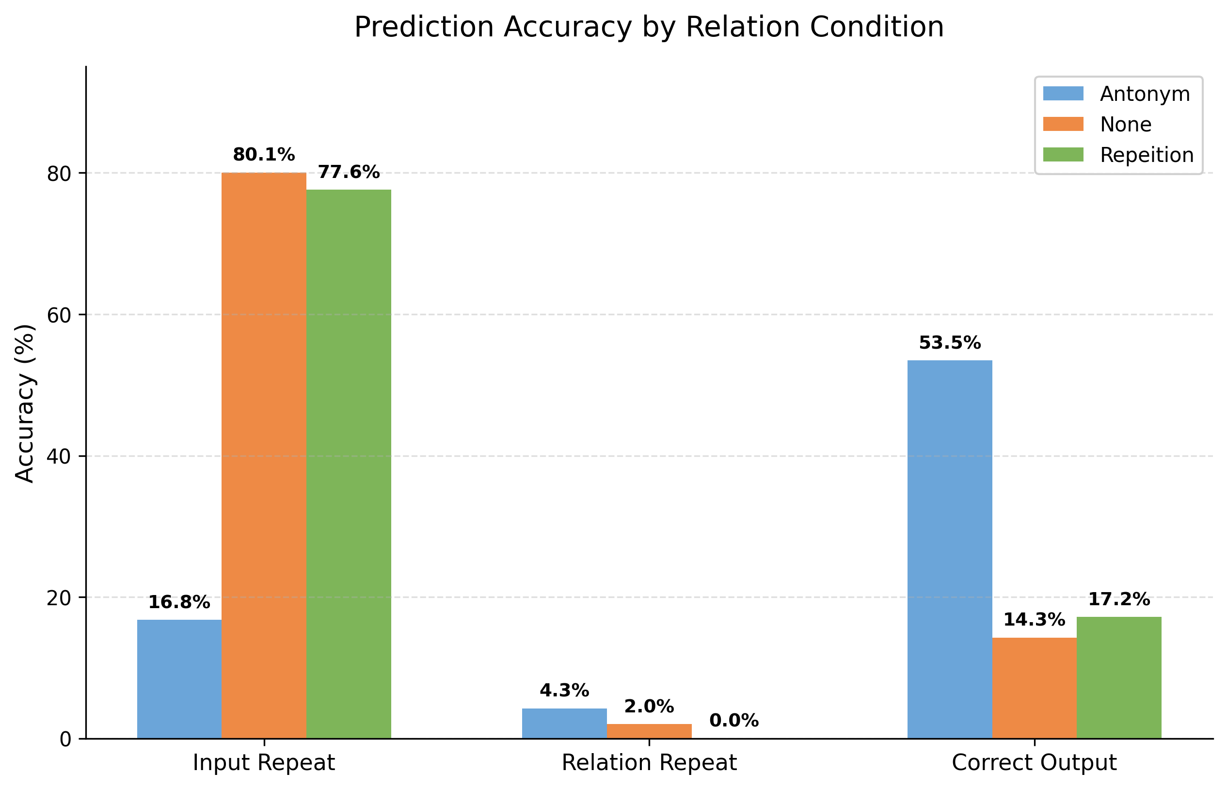
Prediction accuracy across three relation conditions (Antonym, None, Repeat). With the "antonym" relation, the model produces the correct output 53.5% of the time but still falls back to input repeat in 16.8% of cases. Under "none" and "repeat" relations, input repeat dominates at around 80%.
Experiment Details
1. Dataset Split
Following the original paper, the dataset is split into two subsets: one consisting of examples the model answers correctly (used to derive the relation vector) and another consisting of incorrectly answered examples (used to validate generalizability of the relation vector). Also following the paper, the number of prompts used for the clean run and the corrupted run are 100 and 25, respectively.
2. Patching
To derive the relation vector, the activation patching method is employed. The clean run uses the zero-shot prompts as specified above. The corrupt run replaces the relation word “antonym” with “none,” which removes the relation signal while preserving the rest of the prompt structure.
After patching, the Causal Indirect Effect (CIE) is calculated for each attention head. These results are consistent with the original paper: attention heads with strong CIE appear in the middle layers of the model. The relation vector is then constructed by summing the mean output vectors of the top-10 heads (marked with red borders below), after being projected into the hidden state space through their corresponding attention head output matrices.
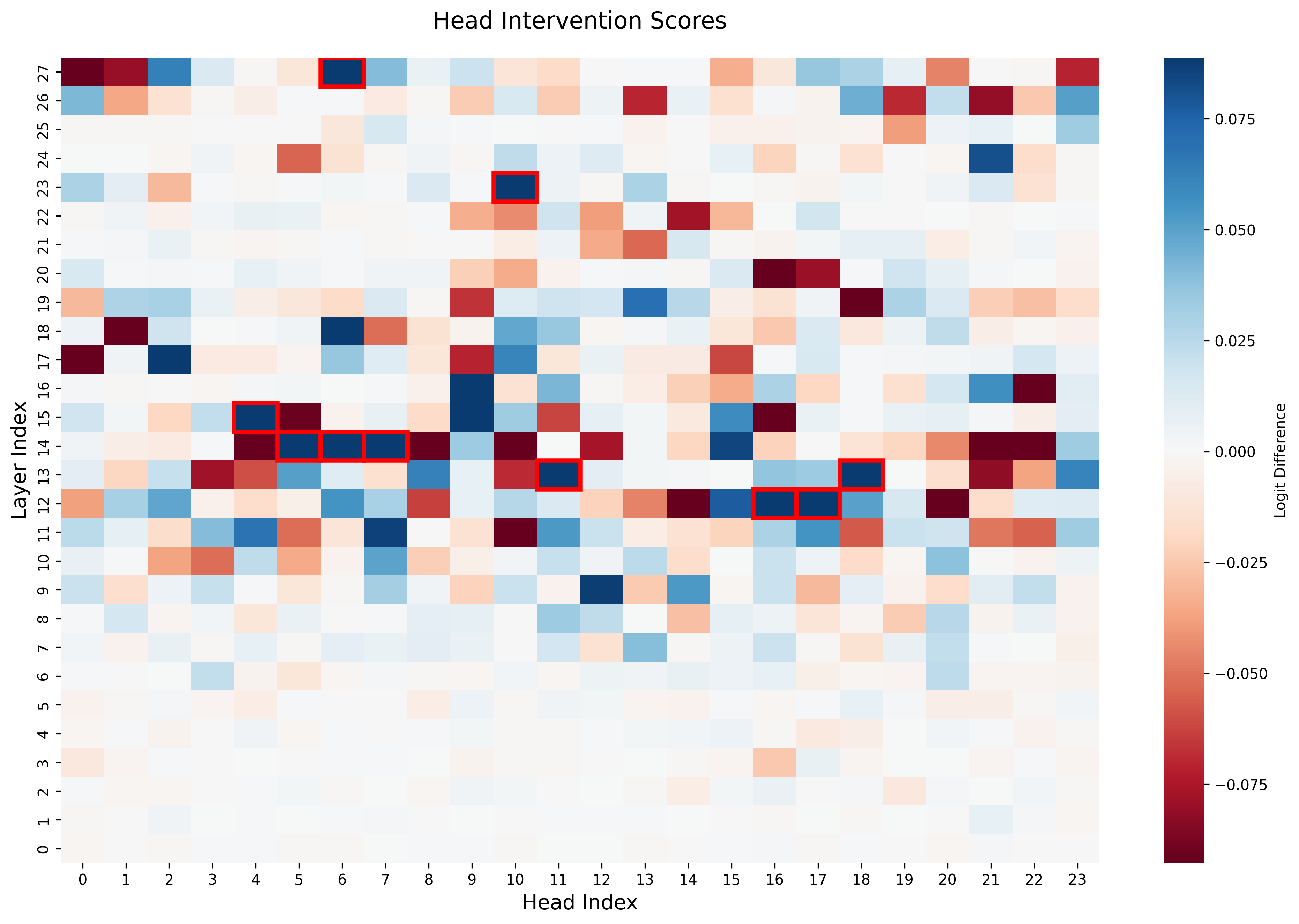
CIE heatmap across all attention heads. The top-10 causally important heads are highlighted with red borders and are concentrated in the middle layers (roughly layers 12–17).
3. Intervention
Intervention experiments were conducted layer-wise in three settings:
-
Normal intervention (
intervention_fig): For the correctly answered subset, the relation is corrupted (replaced with “none”) and the relation vector is added. This is the natural validation setting — it tests whether the relation vector can restore correct behavior when the relation signal has been removed. -
Enforce intervention (
intervention_enforce_fig): For the incorrectly answered subset, the relation is kept intact and the relation vector is added. This setting tests whether the model’s failure on these examples is due to a weak relation signal that can be strengthened. -
Restore intervention (
intervention_restore_fig): For the incorrectly answered subset, the relation is corrupted and the relation vector is added. This setting tests whether the failure can be corrected when the original relation signal is removed and replaced with the relation vector.
Results of Intervention Experiments
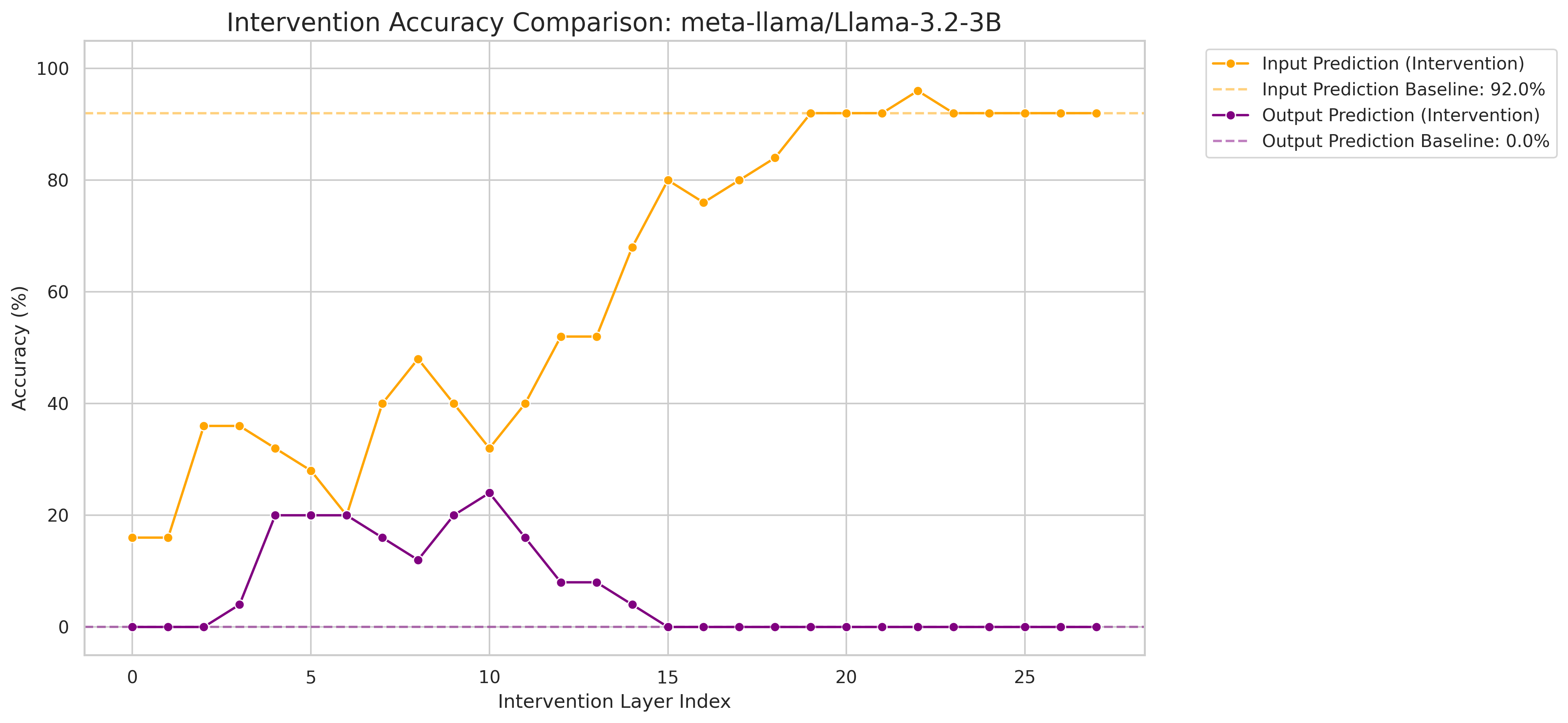
Across the three intervention configurations, the normal intervention showed high restoration of correct answers (over 80%). However, neither the restore setting nor the enforce setting reached above 40% correction on the incorrectly answered subset.
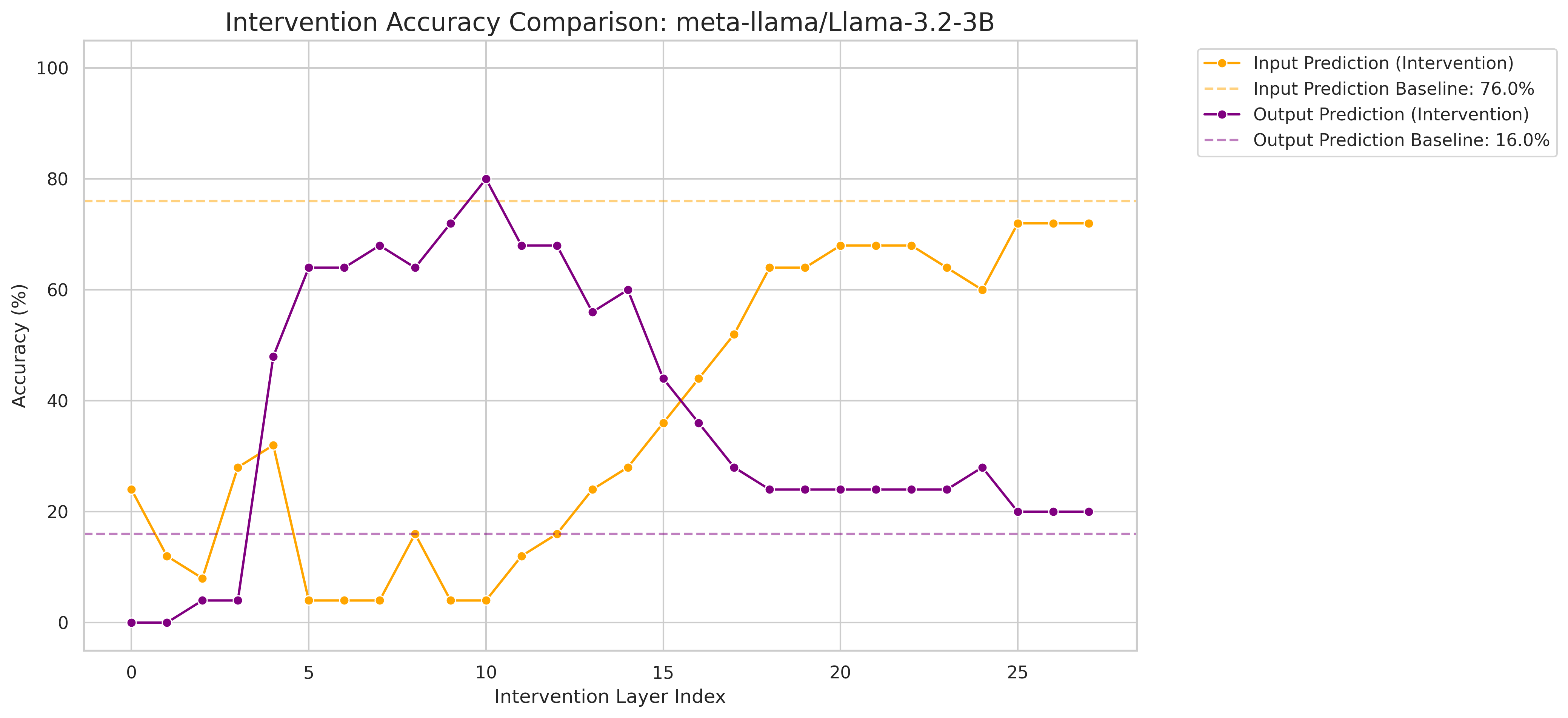
The relation vector restores correct output prediction up to ~80% around the middle layers, while input prediction drops correspondingly.
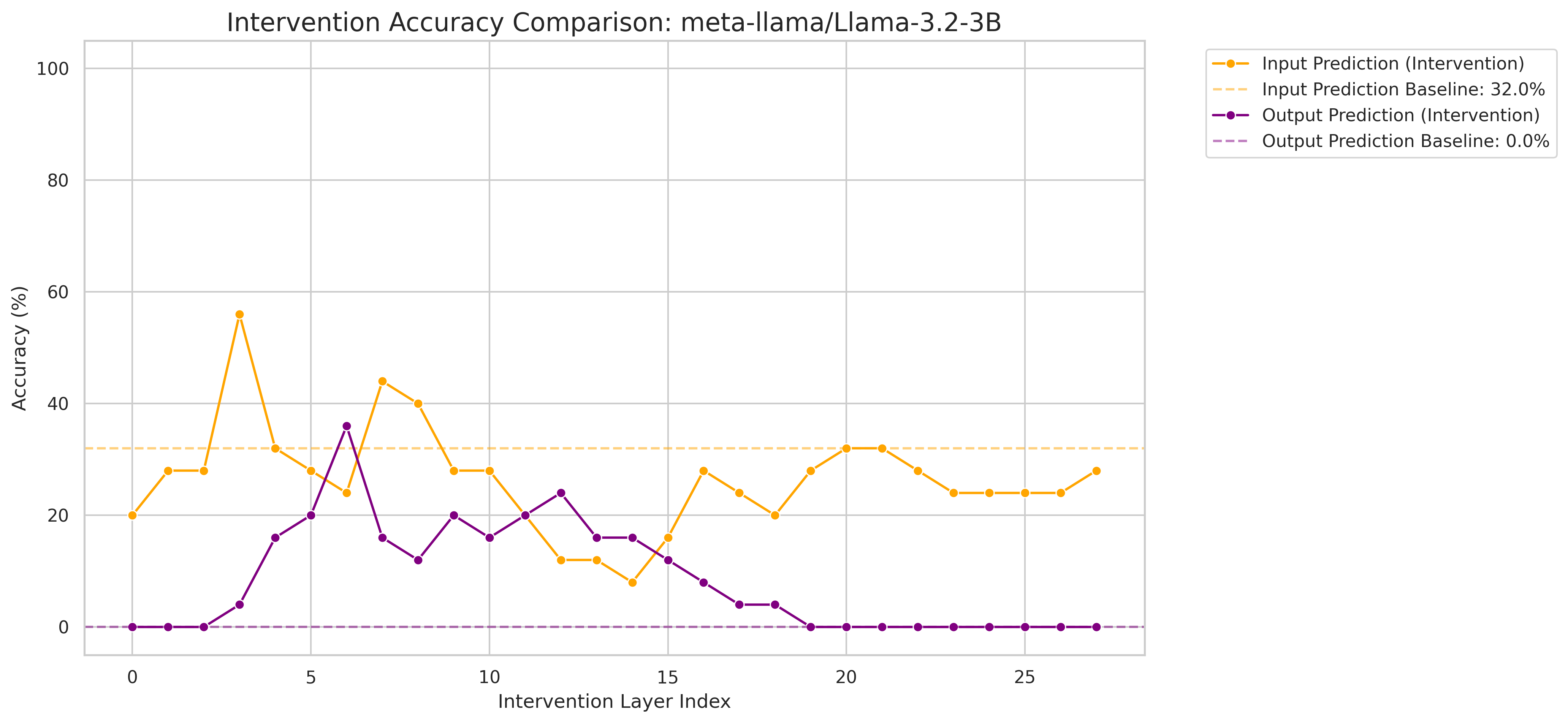
Adding the relation vector on top of the intact relation signal yields only ~35% peak correction. The effect is much weaker than the normal intervention.
Replacing the corrupted relation signal with the relation vector reaches only ~25% peak correction, confirming that the failure mode is not simply a missing relation signal.
Consistent with the original paper, the intervention effect peaks around layer \(L/3\) (approximately layer 9–10 for Llama-3.2-3B with \(L = 28\)), indicating that the relation signal is most effective when injected in the early-to-middle layers of the model.
4. Validation / Generalization
To validate the generalizability of the relation vector, the same intervention experiments at $\frac{L}{3}$ layers, as the paper, are conducted on the prompt formats and different sizes/families of models. The results are shown below:
| Model | Task | Format 1 (`prompt_1e1ef3fe`) | Format 2 (`prompt_f4027ccf`) | ||||||
|---|---|---|---|---|---|---|---|---|---|
| Input prediction | Output prediction | Input prediction | Output prediction | ||||||
| Before (%) | After (%) | Before (%) | After (%) | Before (%) | After (%) | Before (%) | After (%) | ||
| Pythia 2.8B | antonym | 76% | 48% | 20% | 48% | 0% | 0% | 0% | 0% |
| Pythia 6.9B | antonym | 60% | 40% | 8% | 36% | 0% | 0% | 0% | 0% |
| Llama 3.1 8B | antonym | 84% | 0% | 12% | 0% | 0% | 0% | 0% | 0% |
| Llama 3.2 3B | antonym | 76% | 4% | 16% | 72% | 0% | 4% | 0% | 0% |
As seen above, the relation vector is effective in the format 1 for pythia 2.8B, 6.9B and llama 3.2 3B models, but not in the rest of settings. This suggests that the relation vector can be an artifact of the prompt format and the models.
Fallback behavior. The fallback behavior is found during the preliminary experiment. In the prompt format 1, the model highly repeats the input word when the relation is replaced with “none.” But in the prompt format 2, the model does not exhibit this behavior. This suggests that the fallback behavior is not a general property of the model, but rather an artifact of the prompt format.
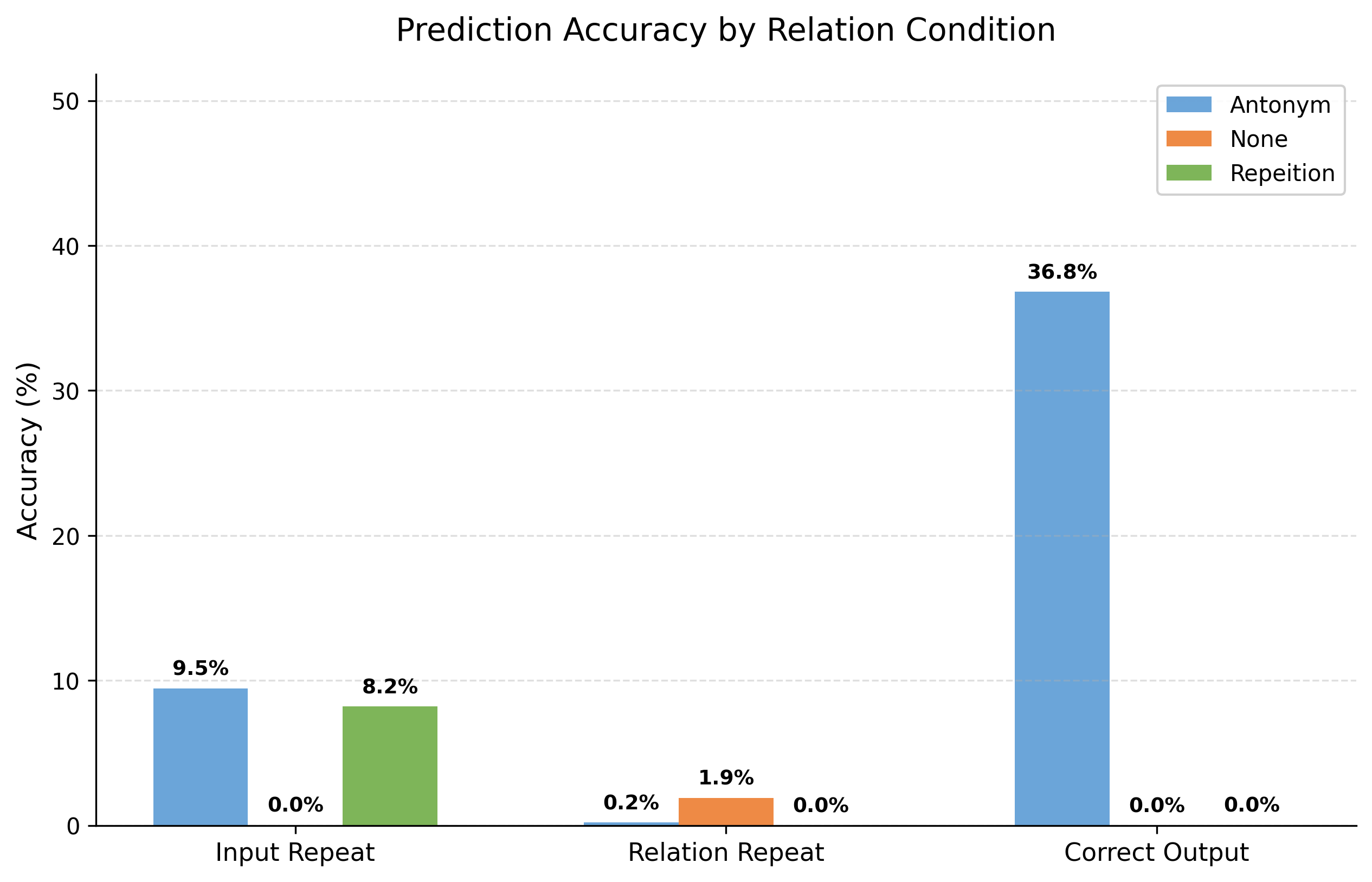
As seen above, the input repetition and output repetition drastically decreased by changing the prompt format.
Implication
Zero-shot inference is a challenging task because it requires the model to understand the relation and the input word in a single pass. The intervention performance varied by prompt format and model size/family, suggesting that a single pass is not enough for the model to understand the relation and the input word.
Given few-shot examplars serve as a guide for the model to understand a task, investigating how the model utilizes the examplars is an intersting next step.
Appendix
This appendix provides the full mathematical notation for the methods used in this post. Appendix A defines the Causal Indirect Effect (CIE) used to identify causally important attention heads, and Appendix B defines the relation vector constructed from those heads.
Appendix A. Causal Indirect Effect (CIE) — Full Notation and Explanation
A.1. Model Setup
We consider an autoregressive transformer language model:
- Model: $f$
- Input prompt: $p$
- Vocabulary: $V$
The model outputs a next-token distribution:
\[f(p) \in \Delta^{|V|}\]For a token $y \in V$:
\[f(p)[y] \in [0,1]\]This is the probability that the model predicts token $y$ given prompt $p$.
A.2. Transformer Internal Notation
The model has $L$ layers.
At layer $\ell$, the hidden state at the final token is:
\[h_\ell \in \mathbb{R}^d\]Each layer is computed as:
\[h_\ell = h_{\ell-1} + m_\ell + \sum_{j=1}^{J} a_{\ell,j}\]where:
- $m_\ell$: MLP output at layer $\ell$
- $a_{\ell,j}$: contribution of attention head $j$ in layer $\ell$
- $J$: number of attention heads per layer
Each attention head output depends on the input prompt:
\[a_{\ell,j}(p)\]A.3. Zero-Shot Inference Setup
We define a relation $r$ (e.g., “antonym”) with dataset:
\[P_r = \{p_i^r\}\]Each prompt is a zero-shot prompt of the form:
\[p_i^r = [\text{Relation: } r, \text{ Input: } x_i, \text{ Output:}]\]where:
- $r$: relation type (e.g., “antonym”)
- $x_i$: input word
- $y_i$: correct answer (not shown in the prompt)
We only keep prompts where the model correctly predicts $y_i$.
A.4. Corrupted (Uninformative) Prompts
We define a corrupted version by replacing the relation with an uninformative one:
\[\tilde{p}_i^r = [\text{Relation: "none"}, \text{ Input: } x_i, \text{ Output:}]\]This removes the relation signal while keeping the prompt structure intact.
A.5. Mean Relation-Conditioned Activation
For each attention head $a_{\ell,j}$, compute:
\[\bar{a}_{\ell,j}^r = \frac{1}{|P_r|} \sum_{p_i^r \in P_r} a_{\ell,j}(p_i^r)\]This is the average activation of head $(\ell,j)$ over clean prompts for relation $r$.
A.6. Intervention (Activation Patching)
We run the model on corrupted prompt $\tilde{p}_i^r$, but replace one head’s activation:
\[a_{\ell,j} := \bar{a}_{\ell,j}^r\]This means that we inject the correct relation-specific signal into a corrupted prompt.
A.7. Causal Indirect Effect (CIE)
The CIE is defined as:
\[\mathrm{CIE}(a_{\ell,j} \mid \tilde{p}_i^r) = f(\tilde{p}_i^r \mid a_{\ell,j} := \bar{a}_{\ell,j}^r)[y_i] - f(\tilde{p}_i^r)[y_i]\]A.8. Interpretation
This measures:
-
the probability of the correct answer after intervention:
\[f(\tilde{p}_i^r \mid a_{\ell,j} := \bar{a}_{\ell,j}^r)[y_i]\] -
the probability of the correct answer without intervention: \(f(\tilde{p}_i^r)[y_i]\)
So:
\[\mathrm{CIE} = \text{(with correct signal)} - \text{(without signal)}\]It quantifies how much this attention head causally contributes to producing the correct answer.
A.9. Average Indirect Effect (AIE)
To aggregate over all corrupted prompts:
\[\mathrm{AIE}(a_{\ell,j}) = \frac{1}{|\tilde{P}_r|} \sum_{\tilde{p}_i^r \in \tilde{P}_r} \mathrm{CIE}(a_{\ell,j} \mid \tilde{p}_i^r)\]This identifies globally important heads for the relation.
Appendix B. Relation Vector Formulation
After computing the average indirect effect (AIE) for every attention head, we select a set of the most causally important heads:
\[A = \{\text{top attention heads ranked by AIE}\}\]Here, $A$ is the set of heads that appear to contribute most strongly to producing the correct answer for relation $r$.
B.1. Relation-Conditioned Mean Activation of a Head
For each selected attention head $a_{\ell,j} \in A$, define its relation-conditioned mean activation for relation $r$ as:
\[\bar{a}_{\ell,j}^r = \frac{1}{|P_r|} \sum_{p_i^r \in P_r} a_{\ell,j}(p_i^r)\]This is the average output of head $(\ell,j)$ over clean prompts for relation $r$.
Interpretation:
- $a_{\ell,j}(p_i^r)$: output of head $(\ell,j)$ on one clean prompt
- $\bar{a}_{\ell,j}^r$: typical head output when the model is processing relation $r$
B.2. Relation Vector Definition
The relation vector for relation $r$ is defined as the sum of these relation-conditioned mean head outputs over the selected causal heads:
\[v_r = \sum_{a_{\ell,j} \in A} \bar{a}_{\ell,j}^r\]This follows the same construction as Equation (5) in the Function Vectors paper, adapted to the zero-shot setting.
B.3. Why This Sum Makes Sense
The formulation relies on the fact that attention head outputs are written in the residual-stream space.
The hidden state is defined as:
\[h_\ell = h_{\ell-1} + m_\ell + \sum_{j=1}^{J} a_{\ell,j}\]Since each $a_{\ell,j} \in \mathbb{R}^d$ already lives in the same residual-stream space as $h_\ell$, their sum also lives in that same space.
Therefore:
\[v_r \in \mathbb{R}^d\]and it can be directly added to hidden states.
B.4. Relation Vector Intervention
Once $v_r$ is constructed, we test it by adding it to a hidden state at layer $\ell$:
\[h_\ell' = h_\ell + v_r\]Equivalently, using the expanded residual-stream form:
\[h_\ell' = h_{\ell-1} + m_\ell + \sum_{j=1}^{J} a_{\ell,j} + v_r\]B.5. Model Output Under Relation Vector Intervention
If we intervene on prompt $p$ by adding $v_r$ at layer $\ell$, the resulting model behavior can be written as:
\[f(p \mid h_\ell := h_\ell + v_r)\]This means:
- run the model on prompt $p$
- at layer $\ell$, replace the hidden state with $h_\ell + v_r$
- continue the forward pass and observe the new output distribution
Enjoy Reading This Article?
Here are some more articles you might like to read next: